Graph Module

Graphs

You can add a graph module to your Subject Viewer layout to allow you to visualize subject data. The LifeOmic Platform uses Plotly for graphing data.

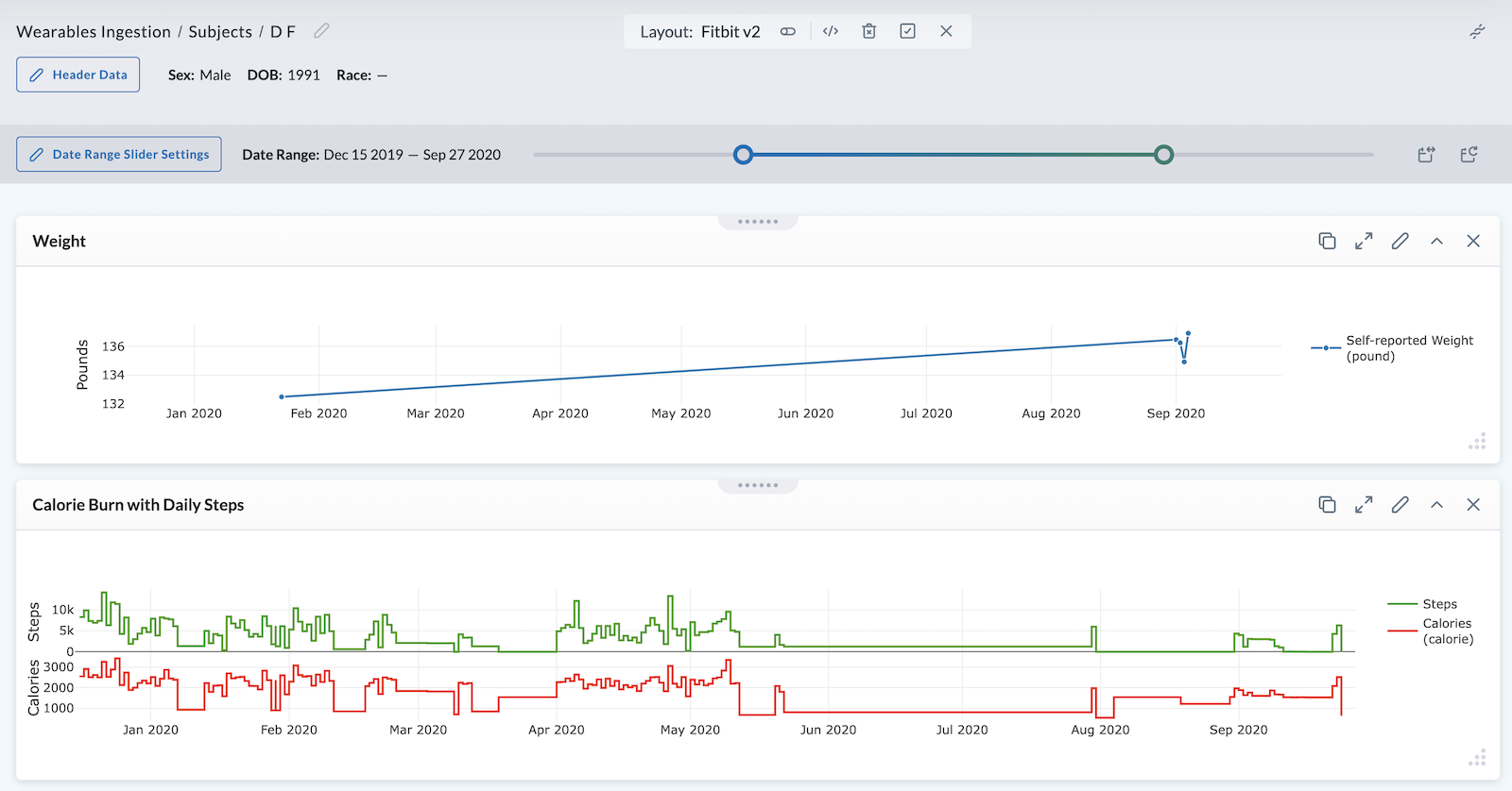
The data displayed is influenced by the timeline slider at the top of the Subject Viewer page. You also can zoom in on a set of data points by hovering your cursor on the graph to access the Mode Bar tools Plotly graphs have to offer, then selecting the Zoom tool, and clicking and dragging to capture the points you wish to zoom in on.

You can configure graphs to show all or a selection of the procedures, observations, and other events.

Adding the Graph Module

1. Begin by following the instructions to Add a Module to a Layout.
2. From the Build Your Own module page, select the Graph tile .
3. Set your graph settings. See detailed section below.
4. Click Apply in Graph Settings. The Subject Viewer layout displays your graph module.
5. To make additional configuration changes, click on the pencil icon to the right of the title to return to Graph Settings.
6. Click the icon in the header to save your layout for future viewing.

note

It is important to complete step 6. You must save the layout itself before you navigate away or the module will not be saved to the layout.

Set Your Graph Settings

When adding a Graph Module to your layout, you'll automatically access the module settings to set the parameters for your graph.

General tab:

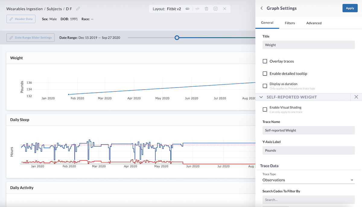
1. Enter the title of your graph in the box under "Title".

2. Click the Add Trace button to continue.

3. Select the traces you wish to plot on your graph. In the example above, the user is plotting self-reported weight generated by a FitBit device. The user has entered "Self-reported Weight" as the Trace Name.

4. Enter a label for your y-axis in the space provided.

5. Choose the Trace Data for your graph. The drop-down menu allows you to select from Observations, Medications, Procedures, Physician Encounters, Conditions, and Goal.

6. Filter your data using search codes. In the example above, the user selected "body weight" to display self-reported weight data generated from a FitBit device.

   • There are multiple codes that can correlate to the same unit of measurement. Wearables from different brands can be coded differently even though the devices are both measuring the same unit. For example, Apple Health weight is a different code than FitBit weight, but they both measure weight.

7. Enter a unit of measure for conversion. In this example, the appropriate unit of measurement is pounds.

8. Use the up and down arrows to select your desired number of points for pagination.

9. If you'd like to add a second trace, click the + Add Trace box. When you are done configuring your graph, click the blue Apply box in the top right corner. There are also additional, advanced ways you can continue to configure your graph, as described below.

Additional Configuration Settings

The General tab contains options for more advanced module configuration. To access the General tab, click on the pencil icon to the right of the title to return to Graph Settings.

Trace Style

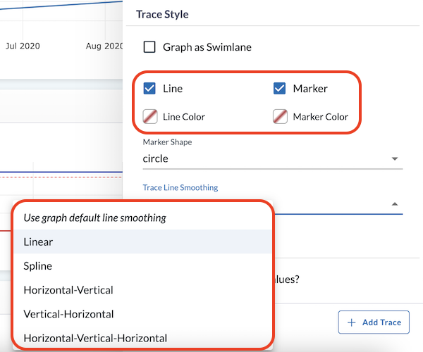
Under the General tab, you can use the Trace Style section to change trace color or data point marker. Click on the color picker to adjust the trace color and marker color.

Graphs have a legend to the right of them, defining what each colored trace or marker represents. These can be toggled on or off by clicking on the trace in the legend (if the layout is saved by clicking the in the header, it will save the graph trace configuration as default). Trace colors and color palettes can be specified, but a color cannot be explicitly tied to a data series. Marker shapes for data points can also be specified.

You can also adjust the smoothing of the graph line in the module settings by selecting your preference from the dropdown menu.

Single events (such as a single dose of medication or a single procedure) are noted on the graph with a single data point. Hovering your cursor on a data point displays more information for that data entry.

Non-quantitative data, such as a diagnosis or medication, is graphed with no y-axis. Events that occur over time (such as a medication taken for a few weeks) will appear as a range. Quantitative data, such as weight or creatinine, has a y-axis.

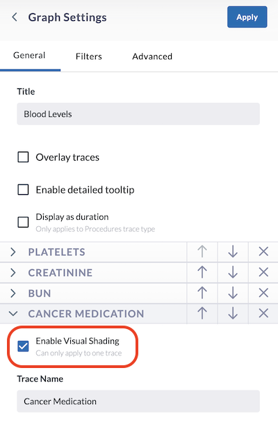
Visual Shading

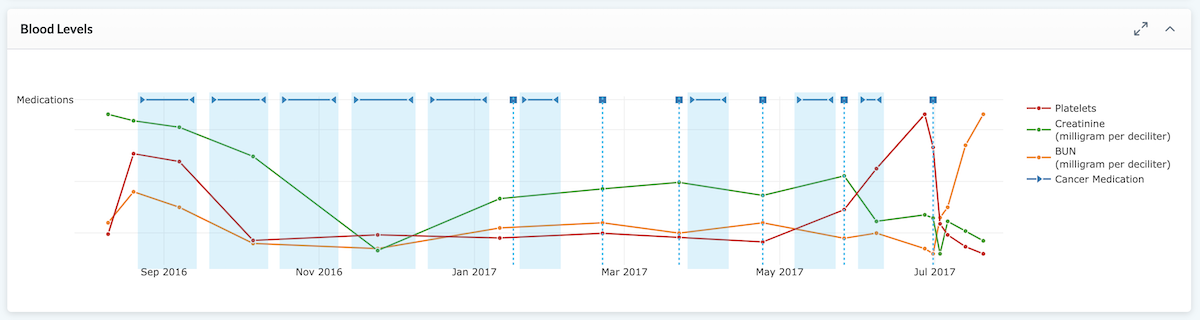
A graph can contain both non-quantitative and quantitative data types. In the image above, the non-quantitative data (cancer medication) is displayed as ranges, but we can enable shading (colored column) for easier viewing of how medication may correlate to various blood levels.

To enable visual graph shading:

1. Enter Layout Edit (click in the header).
2. On the module you wish to add the shading, click the edit icon to enter the Graph Settings.
3. For the data you wish to add shading, click the beside that data name.
4. Check the Enable Visual Shading checkbox. Visual shading can only apply to one trace.
5. Click Apply in the top of the module settings.

Stacked and Layered Graphs

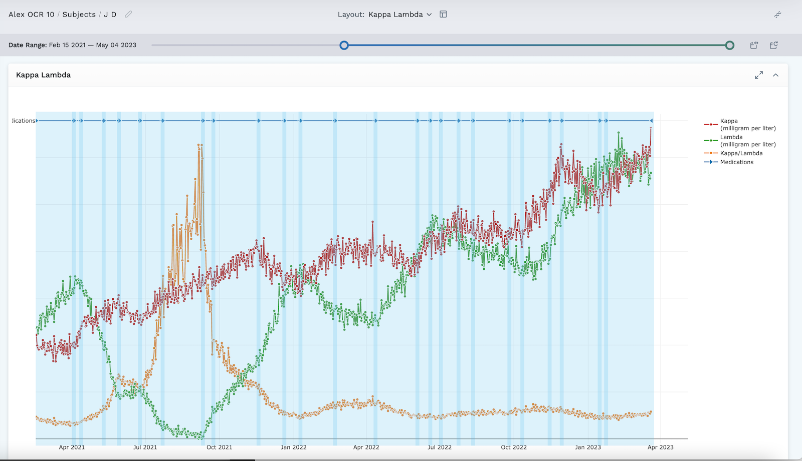
Graphs can be layered or stacked. Layered graphs, such as the one above, occur when different data traces share the same graph, intersecting and overlapping with each other. Data traces set as swimlanes are always displayed at the top of both layered and stacked types of graphs.

Stacked graphs (see image below) occur when different data traces share the same graph but have their own space along the y-axis, not intersecting or overlapping with other traces.

In a stacked graph, Graph tools only work on the trace you are using the tool on, other traces are not impacted.

note

To reset a stacked graph to the default view after using zoom or pan graph tools, double click within that trace's area of the graph.

To create a layered graph, configure the settings so that the traces overlay:

1. Enter Layout Edit (click in the header).
2. On the module you wish to configure, click the edit icon to edit the Graph Settings.
3. Check the Overlay Traces checkbox.
4. Click Apply in the top of the module settings.

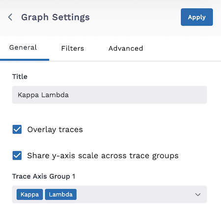
The default graphing of a set of shared observations displays the data independently along the Y axis, with the relative trend not matching exactly across different traces. You can change this and configure the graph so that the traces share a Y axis scale, which can make it easier to directly compare two traces.

To enable a shared Y axis scale across trace groups:

1. Enter Layout Edit (click in the header).
2. On the module you wish to configure, click the edit icon to edit the Graph Settings.
3. Check the Overlay Traces checkbox.
4. Additional options appear. Select the checkbox to Share Y axis scale across trace groups.
5. Under Trace Axis Group 1, use the dropdown arrow to select the desired traces to share the Y axis scale.
6. Click Apply in the top of the module settings.

Detailed Tooltip

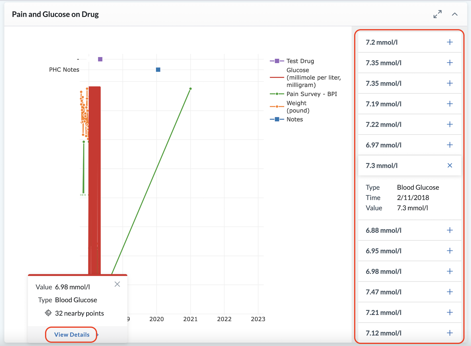
Sometimes a graph has a large number of data points that are grouped so closely together that it can be hard to see individual details. For example, a subject can generate multiple observations during one clinical visit that all have the same date stamp, making them hard to see in a graph. The detailed tooltip feature finds nearby common datapoints, pulls the FHIR data for them, and displays it on the side of the graph for easy viewing.

To enable the detailed tooltip:

1. Enter Layout Edit (click in the header).
2. On the module you wish to add the detailed tooltip, click the edit icon to edit the Graph Settings.
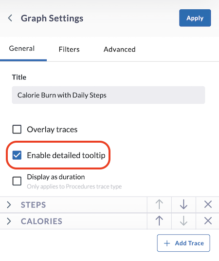
3. Check the Enable Detailed Tooltip checkbox.
4. Click Apply in the top of the module settings.

To use the detailed tooltip:

1. Follow the procedure above to enable the detailed tooltip.
2. Once enabled, click on a datapoint on the graph you wish to see in more detail.
3. If common datapoints are found nearby, the number of datapoints displays above a box that says View Details.
4. Click View Details. The detailed datapoints display in a list in the graph.
5. Click the to display specific data details in a dropdown list.

tip

You can also use the detailed tooltip to favorite specific datapoints in a graph. After clicking on a datapoint in a graph, click on the star to turn it yellow, marking it as a favorite. Visit the detailed section on favoriting data to learn more.

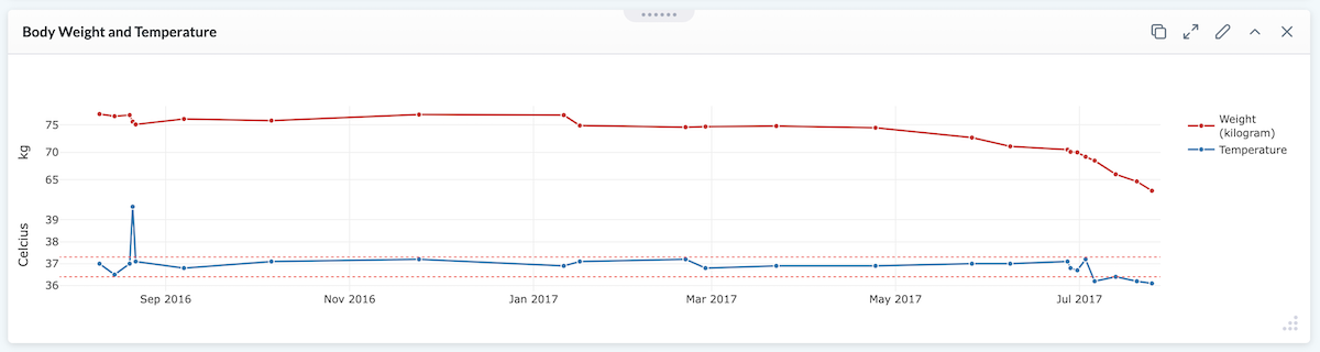
Trace Reference Range

The trace reference range (represented as two red dotted lines shown in the temperature trace in the image above) is a trace level setting and marks the upper and lower limits of normal for that trace. If these values are provided, clicking the checkbox for "Graph with Reference Values?" will configure it to display upper and lower limits of normal.

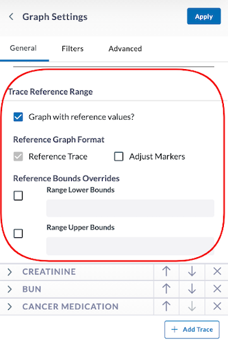
This range can be configured within the layout, allowing the user to dictate what those values are, or the range can come from the FHIR resources (if they are there).

Reference ranges may disappear upon zooming in on the graph.

If the value exceeds the normal range, the data marker shape will be changed to display an arrow up or an arrow down.

Graph Filters and Tagging

Filters tab:

The filters tab allows you to further filter your results.

Tag

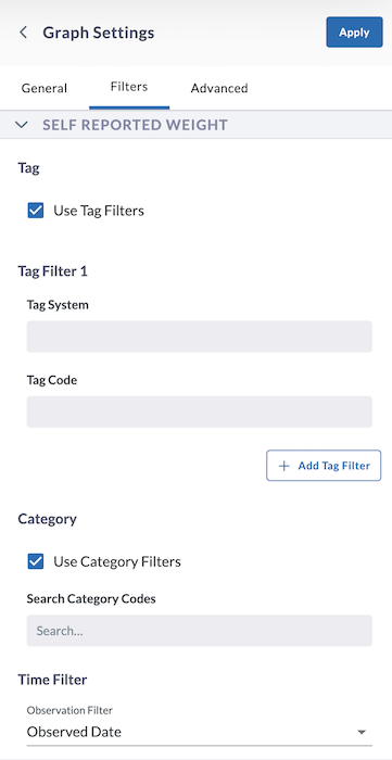
• Use Tag Filters checkbox - After clicking this checkbox, specify the Tag System and Tag Code. You can click the + Add Tag Filter to add more tag filters.

Category

• Use Category Filters checkbox - After clicking this checkbox, search for the Category Code(s) you wish to use.

  Time Filter dropdown - This dictates what time property the data in the graph filters on. Some data types have multiple options to select from here. In the example, the Observation Filter we use is Observed Date.

note

Use the Advanced tab of the Graph Settings to configure specific margin sizes for your graph module.

Graph Tools

Each Graph has two tools at the top right of the module:

• Full Screen - opens the graph as a full screen
• Collapse : - collapses the graph from view

Plotly graphs in the LifeOmic Platform have a mode bar of tools to improve the ease of viewing the displayed data (shown below).

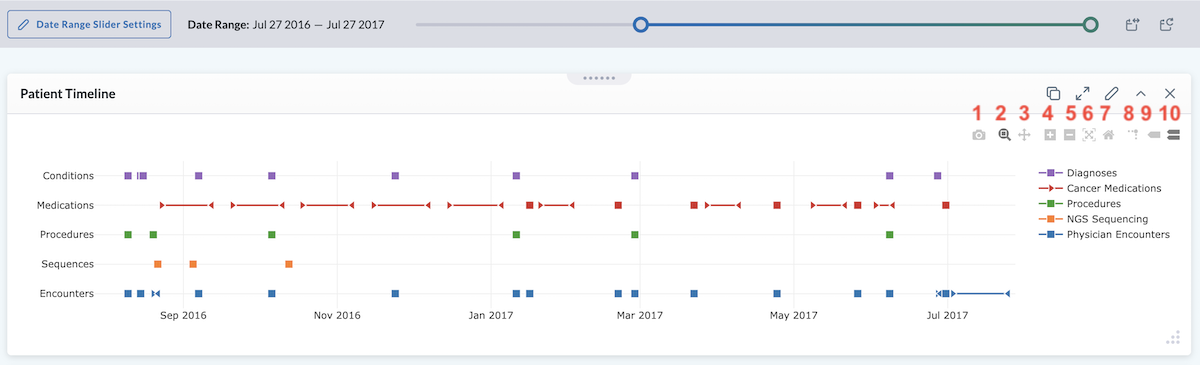
Mode bar graph tools include:

1. Download plot as a PNG
2. Zoom - Zooming can be performed vertically and horizontally. If graphs are stacked, only the one you zoomed in will change. When graphs are layered, all will zoom in. Double clicking within the part you zoomed will reset the vertical
3. Pan - lets you grab and drag the plot to change the date range seen
4. Zoom in - lets you zoom in
5. Zoom out - lets you zoom out
6. Autoscale - reverts after scaling
7. Reset axes - lets up zoom to include your Axes Range, if this has been set. If it has not been set it zooms to a setting that shows all the viewable data.
8. Toggle spike lines – when you hover, this drops a dotted line to the x and y axis to see where it lands
9. Show closest data on hover – shows the one data point you are closest to
10. Compare data on hover – shows all data points when you hover, if you toggle that off you’ll see the single data point that you are closest to